A Bipolar Transmission Line Project -- the TLB Section 2: Design Methodology
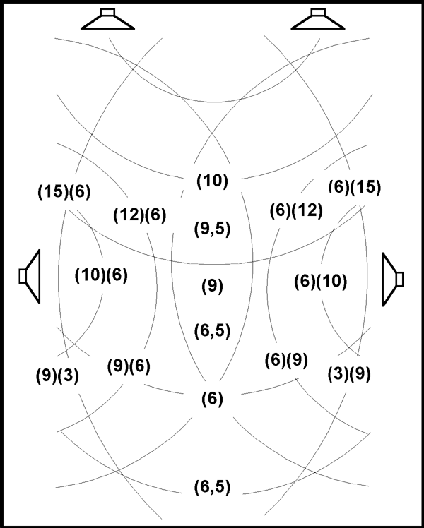
Fig. 2.0 Delayed Source Experiment click image for larger chart	The design of TLB evolved from the attempt to answer the question how do you define the quality of sound stage depth or the concept of imaging. It quickly became apparent that acoustic parameters for these qualities did not exist. Everybody talked about them, but nobody had any data that would compare two speakers for sound stage depth or imaging. Researching the AES papers, I found very few papers that attempted to discus this phenomena. Two papers that attempted to define the perception of directivity were "Extraction of Ambiance Information from Ordinary Recordings" by E.R. Madsen and "Pinna Transformations and Sound Reproductions" by C.A. Puddie Rodgers. Madsen used the concept that 'ambiance is that characteristic of space in which the original recording was made and is represented by the reverberation components of the sound field in that space'. This concept was first investigated by H. Haas as part of the investigation of intelligibility of speech under the influence of echo, for whom the Haas effect is named. The theoretical psychoacoustic concepts are summed in a discussion of an experimental recreation of ambience from a conventional stereo recording via a delay mechanism fed to two side speakers, Fig. 2.0. I decided to repeat this experiment and to attempt to quantify the reverberant field by MLS pulse measurements using Laud.
Short Course in PsychoAcoustics To understand the results, we have to summarize some of the concepts established by Haas. In a concert hall, sound information is received from widely separated directions: direct sound information, the first sound wave to reach the listener's ears from the source. an infinite number of reflected sound waves following immediately after the direct sound; the directional quality is described as diffused.
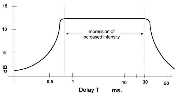
Fig. 2.1 Amplitude vrs Delay Directivity Function click image for larger chart	The subjective effect for the listener upon receiving two identical pulsed sounds may be a simple sum, but it also depends upon the delay between the pulses. If the sources are spaced in direction as well as time, then a sound image with characteristic direction in 3D space is the result of this integration. The virtual image is stable against increases in intensity for the second source only if the intensity for the second source does not exceed the threshold as plotted vs. delay in Fig. 2.1 characterized as the Haas Effect: the reception of two sounds identical except for delay, results in the impression of a single louder sound from a characteristic direction, unless the second sound exceeds the threshold shown by the curve. For longer delays (>30 ms), a tendency to hear a double sound is observed, and for shorter delays (< 1 ms), the directionality is delay dependent. For medium delays (1-30 ms), the localization is fixed on the first received sound with the second enhancing the loudness of the first. Thus by classifying the delay of the reflected sound we can establish the directivity of the apparent source
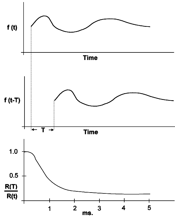
If the two pulses differ by a certain time delay, the displacement results in an incoherence that may be identified as a casual element for the subjective effects. In discriminating among otherwise identical sound pulses, incoherence to a greater or lesser degree describes whether the signals may be identified as a single signal to a lesser or greater degree. Signals coherent in time but not in direction are heard as one from a ficticious or phantom source that is localized between the two sources at a place dependent upon the relative intensities of the sources. Signals coherent in direction but not in time are heard essentially as one, with the delayed signal, when audible, being heard much more weakly. Signals incoherent in both time and direction are heard as not localized, neither from source nor from a large range of angles in space, ie as a diffused sound.
Fig. 2.2 Autocorrelation function Construction of the Autocorrelation Measure of Coherence click image for larger chart	The degree of coherence in time is strongly dependent upon delay, but the form of sound is also a factor.This is readily seen if coherence is expressed in terms of an autocorrelation function.For pulselike signals, this function R(t) is simply the sum of the products of the amplitudes for staggered replicas of the signal, and is regarded as a function of the extent of stagger, the delay t. . It is apparent that the degree of coherence decreases as the delay t departs from zero and that this drop off in coherence will be more rapid the more the signal is characterized by short-time detail
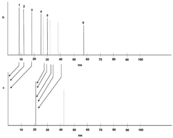
Collapse of the Reverberant Field For a complex train of pulses the above can be summarized as: The reproduced physical pulse train, top graph Fig. 2.3, shows the reverberant field. It is perceived by the ear/brain interface as: Reverberant field 8 - 20 ms collapsing into the primary pulse. Reverberant field 20 - 40 ms collapsing into the secondary pulse, defined by the Haas effect.. Reverberant field > 40 ms perceived as an echo. The classification of the reverberant sound field outlined above gives us the tools to examine the MLS pulse field produced by Fig. 2.0 setup. Since the delay feeding the side speakers could be varied in the range of 0 — 100 ms and the amplitude controlled separately from that of the front speakers, the subjective sound stage and localization could be correlated to that of the delay produces sound field. Laud instrumentation permitted the isolation of the reverberant pulse train and via a FFT transform the comparison of the frequency response to that of the original MLS source. Thus the examination of a delayed or reverberant signal in the time domain defined the subjective phenomena of the sound stage depth and of the virtual image.	Fig. 2.3 Reverberant Pulse Field
Once a reference set of data established by the synthetic delay was on hand, a comparison to that of the monopole TL radiation pattern could be made. The next step was the attempt to examine the dipole pattern. Unfortunately the TL is not amiable to a dipole configuration, the terminal signal amplitude and thus the low frequency response collapses, thus the bipole configuration was attempted. This worked and the rest of the document describes the TLB configuration. The fundamental principle was that the bipole recreated the complex waveform interaction of the reverberant field that was synthesized by the external delay, by reflections from the side-walls, the back-wall and the ceiling. The reverberant fields were remarkably similar to that produced by the synthesized delay. This is the basis for the requirement that the TLB be placed away from the room boundaries. The sound field produced of course is a function of the quality of the recording. Multi-mic mixed recordings are usually revealed to produce a flat sound stage, while the minimalist stereo mike in the hands of a knowledgeable recording engineer produces an amazingly realistic recreation of the original. The sound stage produced by the TLB stretches to the wall boundaries and is very deep to the rear of the speakers. The virtual image is solid with frequency and amplitude. The speaker also has a very wide 'sweet spot' about 3 ft of the central axis. The most appealing quality to me is the ability to reproduce very soft passages without veiling. This is related to an interesting observation, with your eyes closed to walk up to and beyond the horizontal axis of the speakers and perceive very little change in amplitude. The bipole radiation field is very homogeneous.
[ Contents | Introduction | Methodology | Radiation Response | Transient Response | Frequency Response | Construction ]